In this chapter we present the results of benchmarking SWAMP against the two most used computer models for
sound propagation in underwater acoustics.
The first model, the Range-dependent Acoustic Model (RAM)
by Collins, is based on the split-step Padè solution
of the parabolic equation. The
split-step Padè algorithm employs a rational function approximation of the
differential operators and is claimed to be the most efficient PE algorithm
that has been developed. It allows
larger range steps in comparison with
other PE models for a marching-in-range procedure that gives it much better computational stability and
performance in time. The second
model, KRAKEN by Porter, represents the normal mode model with a
finite-difference approach for solution of the depth-separated modal
equation. KRAKEN computes the solution
of range-dependent problems in the coupled or adiabatic approximation.
The first benchmark problem contains
range-dependent bathymetry and a sound speed profile, which varies with
depth. The ocean bottom profile
(bathymetry) is shown in Figure 4.1. It
includes a range-independent environment with a 1000 meter deep water-column
from 0 to 35 km and a relatively steep up-sloping ocean bottom from 35 to 45
km with depth changes from 1000
m to 200 m. The sound speed profile is
shown in Figure 4.2. The environment has a bottom duct. The receiver depth is
30 m. The source is placed at depths
of 25 m and 400 m. The test frequency
is 100 Hz.
Transmission
loss (![]() )
is the standard
normalized measure of the change in signal strength with range in underwater
acoustics. It is defined as the ratio in decibels between the acoustic
intensity at a receiver point and the intensity at 1-m distance from the
source:
)
is the standard
normalized measure of the change in signal strength with range in underwater
acoustics. It is defined as the ratio in decibels between the acoustic
intensity at a receiver point and the intensity at 1-m distance from the
source:
![]() (1)
(1)
In
Eq. (1) the fact that the intensity is proportional to the square of the
pressure amplitude has been used.
Usually, the reference pressure at 1-m distance is determined by the approximation for a source in free space:
![]() , (2)
, (2)
because
all waveguide effects start at
distances not less than the wavelength. Sometimes a minus sign is put in front
of the logarithm function in (1), so the transmission loss becomes a positive value for the far field. All the transmission plots in this paper
have been calculated using formula (1), so that smaller values of the
transmission loss (large negative values) correspond to smaller signals, i.e., larger loss in the
propagation to the given point.
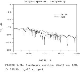
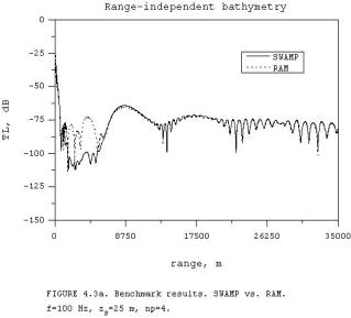 Figures
4.3(a) and 4.3(b) show plots of the transmission
loss versus range obtained with SWAMP (solid line) and RAM (dashed
line). The two parts of Fig. 4.3 - (a)
and (b) - represent the same continuous calculations but are separated into the
range-independent part of the propagation path (up to 35 km) and the range-dependent one (35-50 km) for
better visibility. The source depth is
25 m. The number of Padè terms np in the rational function
approximation of the differential operator in the PE-model RAM is 4. Figure 4.3 (a) shows no visible
discrepancies in the match between the
transmission loss predicted by SWAMP and RAM for the range-independent
bathymetry starting around 8 km. The later plots of benchmarking SWAMP
with the other propagation model, KRAKEN,
show a good agreement in the near field. Thus, mismatching between SWAMP
and RAM results in the near zone (up to 8 km) can be probably related to the details of a new self-starter for a point
source implemented in RAM. RAM employs
an indirect method for taking the continuum modal spectrum into account, which is important in the near
field. SWAMP does not take the continuum modal spectrum into account. It can also contribute into the observable
difference in the transmission loss prediction in the near zone. The benchmark results for the
range-dependent bathymetry shown in Fig. 4.3(b) are in quite good agreement, which can not be expected to be perfect
because of the different types of implemented approximations and a fair number
of ambiguous input parameters required for any PE model, such as a number
of the Padè terms, the type of stability constraints, the reference sound
speed, the false bottom depth, the vertical sampling mesh, etc.. Both models have used the same minimum marching step size in
range - 10 m. It is important to note
that the steep up-slope bottom problems are considered to be among the most difficult problems for
numerical simulation because high-order modes become lost. The loss of
modes is equivalent to the energy transfer into the bottom layers. This effect can be accurately accounted only
by including the continuum modal spectrum. The benchmark results for the
down-slope bottom and more gradual up-slope
bottom cases show the much better agreement between the two models.
Figures
4.3(a) and 4.3(b) show plots of the transmission
loss versus range obtained with SWAMP (solid line) and RAM (dashed
line). The two parts of Fig. 4.3 - (a)
and (b) - represent the same continuous calculations but are separated into the
range-independent part of the propagation path (up to 35 km) and the range-dependent one (35-50 km) for
better visibility. The source depth is
25 m. The number of Padè terms np in the rational function
approximation of the differential operator in the PE-model RAM is 4. Figure 4.3 (a) shows no visible
discrepancies in the match between the
transmission loss predicted by SWAMP and RAM for the range-independent
bathymetry starting around 8 km. The later plots of benchmarking SWAMP
with the other propagation model, KRAKEN,
show a good agreement in the near field. Thus, mismatching between SWAMP
and RAM results in the near zone (up to 8 km) can be probably related to the details of a new self-starter for a point
source implemented in RAM. RAM employs
an indirect method for taking the continuum modal spectrum into account, which is important in the near
field. SWAMP does not take the continuum modal spectrum into account. It can also contribute into the observable
difference in the transmission loss prediction in the near zone. The benchmark results for the
range-dependent bathymetry shown in Fig. 4.3(b) are in quite good agreement, which can not be expected to be perfect
because of the different types of implemented approximations and a fair number
of ambiguous input parameters required for any PE model, such as a number
of the Padè terms, the type of stability constraints, the reference sound
speed, the false bottom depth, the vertical sampling mesh, etc.. Both models have used the same minimum marching step size in
range - 10 m. It is important to note
that the steep up-slope bottom problems are considered to be among the most difficult problems for
numerical simulation because high-order modes become lost. The loss of
modes is equivalent to the energy transfer into the bottom layers. This effect can be accurately accounted only
by including the continuum modal spectrum. The benchmark results for the
down-slope bottom and more gradual up-slope
bottom cases show the much better agreement between the two models.

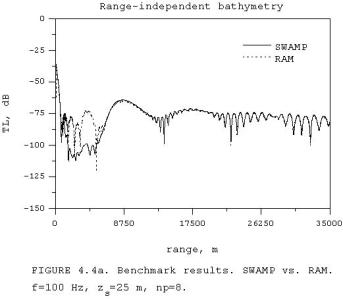 Fig.
4.4 shows the use of more Padè terms in
RAM, namely np=8, gives better
agreement for the up-slope propagation
as is indicated in Fig. 4.4 (b). The phenomenon responsible for a more
oscillatory interference pattern for the PE results is probably related to the
so-called Gibbs oscillations, since different quantities are conserved across
horizontal and vertical interfaces in
PE modeling with sloping interfaces.
The basis of the problem is the choice of the vertical interface
boundary conditions for range-dependent problems. It was shown that solutions
which match pressure alone or only particle velocity show serious
deficiencies. Fairly accurate solutions
for most PE problems in ocean acoustics can be obtained by conserving
Fig.
4.4 shows the use of more Padè terms in
RAM, namely np=8, gives better
agreement for the up-slope propagation
as is indicated in Fig. 4.4 (b). The phenomenon responsible for a more
oscillatory interference pattern for the PE results is probably related to the
so-called Gibbs oscillations, since different quantities are conserved across
horizontal and vertical interfaces in
PE modeling with sloping interfaces.
The basis of the problem is the choice of the vertical interface
boundary conditions for range-dependent problems. It was shown that solutions
which match pressure alone or only particle velocity show serious
deficiencies. Fairly accurate solutions
for most PE problems in ocean acoustics can be obtained by conserving ![]() , which is energy conserving in a forward sense for
horizontally propagating sound. But one still has to be aware of Gibbs
oscillations. More numerical modeling with different RAM input parameters is
required to understand the correct mechanism causing these additional wiggles
in the interference pattern.
, which is energy conserving in a forward sense for
horizontally propagating sound. But one still has to be aware of Gibbs
oscillations. More numerical modeling with different RAM input parameters is
required to understand the correct mechanism causing these additional wiggles
in the interference pattern.
The computational time taken by SWAMP to do the
calculations presented in Fig. 4.3 and 4.4 on a Pentium-133 is 53 seconds. For RAM, the computational time is very
dependent on the number of Padè terms.
It takes 2 minutes 8 seconds to
perform the calculations with np=4
(Figure 4.3) and 4 minutes 14 seconds
with np=8 (Figure 4.4).
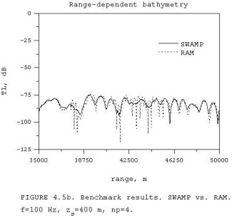
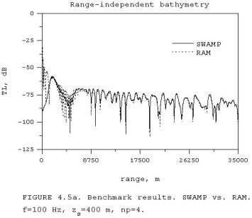
Wide-angle propagation is
illustrated in Fig. 4.5(a),(b), when the source is placed at 400 m depth and
the transmission loss is measured at 30 m depth. The fit between the two models is amazingly good.
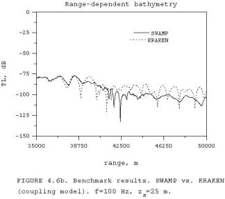
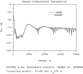 The benchmark results for SWAMP and the
coupled normal mode model KRAKEN are
presented in Fig. 4.6(a) and (b).
As was pointed out before, we
can see good agreement for the near zone which
was not the case for RAM. All
the KRAKEN results were obtained on an
SGI computer. Therefore I can
not make any reasonable computational
time comparisons for the range-independent case. KRAKEN uses a
finite-difference scheme for the solution of the modal equation, which slows it down considerably relative to
SWAMP. KRAKEN was not intended for
range dependent calculations with the coupled mode approach, so it is very
difficult to run for range-dependent
cases. One has to create environmental input files for as many
range-independent subregions as one wants to have. There is no literature on an optimal procedure for
the determination of optimal step-size in range for this model. The adiabatic
approximation for the KRAKEN model produces very poor results for this type of
environment after proceeding half-way
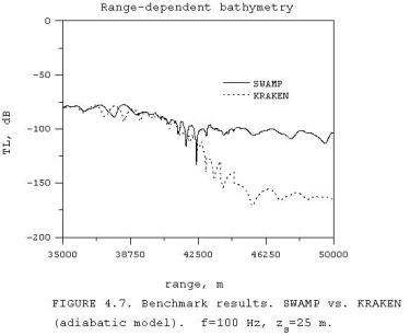
through the sea mount region (after 42 km) as can be seen in Fig. 4.7.
The benchmark results for SWAMP and the
coupled normal mode model KRAKEN are
presented in Fig. 4.6(a) and (b).
As was pointed out before, we
can see good agreement for the near zone which
was not the case for RAM. All
the KRAKEN results were obtained on an
SGI computer. Therefore I can
not make any reasonable computational
time comparisons for the range-independent case. KRAKEN uses a
finite-difference scheme for the solution of the modal equation, which slows it down considerably relative to
SWAMP. KRAKEN was not intended for
range dependent calculations with the coupled mode approach, so it is very
difficult to run for range-dependent
cases. One has to create environmental input files for as many
range-independent subregions as one wants to have. There is no literature on an optimal procedure for
the determination of optimal step-size in range for this model. The adiabatic
approximation for the KRAKEN model produces very poor results for this type of
environment after proceeding half-way
through the sea mount region (after 42 km) as can be seen in Fig. 4.7.