Representing the Input Space at the Hidden Units

After training a network, each hidden unit  generates a decision separation in the input space , i.e. separates some inputs from others. Different activation functions would result in different separation boundary characteristics. For a hidden unit with sigmoidal activation function, the separation will be a line with two dimensional inputs and a plane with three dimensional inputs.

Since the threshold  (bias ) of units can be trained, the separation boundary will be shifted depending on the threshold value of the unit, and the computation done at the output layer. Since the aim is only to visualize the hidden layer, information coming from the output layer should not be included. Eventually, the real boundary will be different for each output unit.

Therefore, the activation levels of the hidden unit will be given for all possible points in input space, by changing the input variables, along their respective ranges and plotting the activation level of the hidden unit.

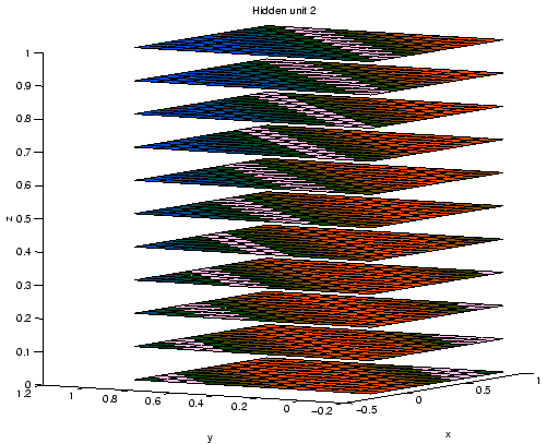
Here the dimensionality of the problem will be of importance. For networks with two inputs, we will have a plane where the activation of the hidden unit varies. In this case, it is clearer to represent the activations as elevations in the third dimension, i.e. z-axis, still colored for better visualization as seen in Figure 3 created by file Tools/InputSpace2D.m described in Section 4.2.1.

  

Figure 3: Variations in the hidden unit activation, when 2 inputs are swept across their range for the 2 bit XOR problem.

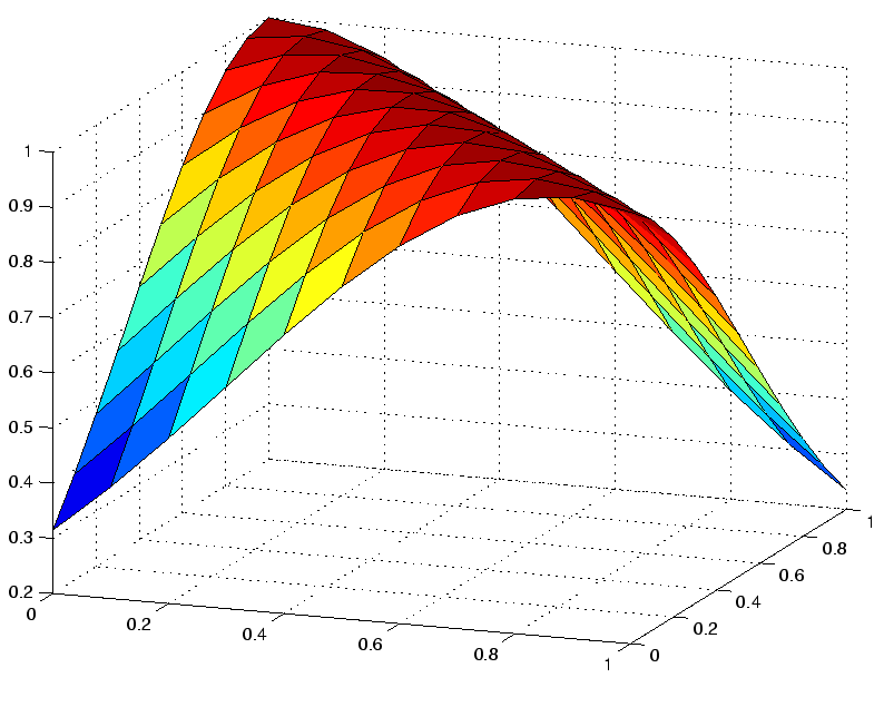
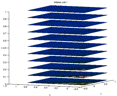
For networks with three inputs, we will have a quadrangular prism⁸ where the activation of the hidden unit varies. Here, we are left with representing the activation of the unit only by colors, since we cannot visualize it by introducing a new dimension (the 4^th dimension). The cube will be represented as colored slices to show the activations as seen in Figure 4 created by file Tools/InputSpace3D.m described in Section 4.2.1.

  

Figure 4: Variations in the hidden unit activation, when 2 inputs are swept across their range.

Looking at the separation boundary of each hidden unit might be useful in understanding the functionality of the output layer of the network (see files in Section 4.2.1 for details about implementation).